How to calculate confidence intervals for ratios?

Question

Consider an experiment that outputs a ratio $X_i$ between 0 and 1. How this ratio is obtained should not be relevant in this context. It was elaborated in a previous version of this question, but removed for clarity after a discussion on meta.

This experiment is repeated $n$ times, while $n$ is small (about 3-10). The $X_i$ are assumed to be independent and identically distributed. From these we estimate the mean by calculating the average $\overline X$, but how to calculate a corresponding confidence interval $[U,V]$?

When using the standard approach for calculating confidence intervals, $V$ is sometimes larger than 1. However, my intuition is that the correct confidence interval...

1. ... should be within the range 0 and 1
2. ... should get smaller with increasing $n$
3. ... is roughly in the order of the one calculated using the standard approach
4. ... is calculated by a mathematically sound method

These are not absolute requirements, but I would at least like to understand why my intuition is wrong.

Calculations based on existing answers

In the following, the confidence intervals resulting from the existing answers are compared for $\{X_i\} = \{0.985,0.986,0.935,0.890,0.999\}$.

Standard Approach (aka "School Math")

$\overline X = 0.959$, $\sigma^2 = 0.0204$, thus the 99% confidence interval is $[0.865,1.053]$. This contradicts intuition 1.

Cropping (suggested by @soakley in the comments)

Just using the standard approach then providing $[0.865,1.000]$ as result is easy to do. But are we allowed to do that? I am not yet convinced that the lower boundary just stays constant (--> 4.)

Logistic Regression Model (suggested by @Rose Hartman)

Transformed data: $\{4.18,4.25,2.09,2.66,6.90\}$ Resulting in $[0.173,7.87]$, transforming it back results in $[0.543,0.999]$. Obviously, the 6.90 is an outlier for the transformed data while the 0.99 is not for the untransformed data, resulting in a confidence interval that is very large. (--> 3.)

Binomial proportion confidence interval (suggested by @Tim)

The approach looks quite good, but unfortunately it does not fit the experiment. Just combining the results and interpreting it as one large repeated Bernoulli experiment as suggested by @ZahavaKor results in the following:

$985+986+890+935+999 = 4795$ out of $5*1000$ in total. Feeding this into the Adj. Wald calculator gives $[0.9511,0.9657]$. This does not seem to be realistic, because not a single $X_i$ is inside that interval! (--> 3.)

Bootstrapping (suggested by @soakley)

With $n=5$ we have 3125 possible permutations. Taking the $\frac{3093}{3125} = 0.99$ middle means of the permutations, we get $[0.91,0.99]$. Looks not that bad, though I would expect a larger interval (--> 3.). However, it is per construction never larger than $[min(X_i),max(X_i)]$. Thus for a small sample it will rather grow than shrink for increasing $n$ (--> 2.). This is at least what happens with the samples given above.

Answer 1

First, to clarify, what you're dealing with is not quite a binomial distribution, as your question suggests (you refer to it as a Bernoulli experiment). Binomial distributions are discrete --- the outcome is either success or failure. Your outcome is a ratio each time you run your experiment, not a set of successes and failures that you then calculate one summary ratio on. Because of that, methods for calculating a binomial proportion confidence interval will throw away a lot of your information. And yet you're correct that it's problematic to treat this as though it's normally distributed since you can get a CI that extends past the possible range of your variable.

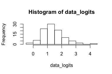
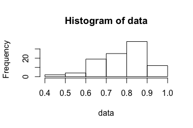
I recommend thinking about this in terms of logistic regression. Run a logistic regression model with your ratio variable as the outcome and no predictors. The intercept and its CI will give you what you need in logits, and then you can convert it back to proportions. You can also just do the logistic conversion yourself, calculate the CI and then convert back to the original scale. My python is terrible, but here's how you could do that in R:

set.seed(24601)
data <- rbeta(100, 10, 3)
hist(data)

data_logits <- log(data/(1-data)) 
hist(data_logits)

# calculate CI for the transformed data
mean_logits <- mean(data_logits)
sd <- sd(data_logits)
n <- length(data_logits)
crit_t99 <- qt(.995, df = n-1) # for a CI99
ci_lo_logits <- mean_logits - crit_t * sd/sqrt(n)
ci_hi_logits <- mean_logits + crit_t * sd/sqrt(n)

# convert back to ratio
mean <- exp(mean_logits)/(1 + exp(mean_logits))
ci_lo <- exp(ci_lo_logits)/(1 + exp(ci_lo_logits))
ci_hi <- exp(ci_hi_logits)/(1 + exp(ci_hi_logits))

Here are the lower and upper bounds on a 99% CI for these data:

> ci_lo
[1] 0.7738327
> ci_hi
[1] 0.8207924

Answer 2

You might want to try resampling/bootstrapping. Let's look at the simple case you mentioned.

With 3 data points of 0.99, 0.94, and 0.94, you wouldn't even do the resampling because you can just list out all 27 possible permutations, find the mean in each case, and then sort the means.

If you create the list and take the middle 25 observations, you have a $25/27=$ 92.6% confidence interval of [0.9400, 0.9733]. If you want to increase the confidence to $26/27=$ 96.3%, you have two one-sided choices of intervals. Either [0.9400, 0.9733] or [0.94, 0.99].

I assume your $n$ will be much greater than 3, so you will resample with replacement. Say you do this 1000 times. Then find the mean in each case. From the set of 1000 means, take the middle 950 values. The lowest and highest values of this subset form the 95% confidence interval.

The question here: How do we create a confidence interval for the parameter of a permutation test? gives more detail, including some R code.

Answer 3

Binomial confidence intervals have been the subject of statistician debates for a long time. Your problem considers a less than 100% ratio, but it becomes even more problematic if we use 100%. One insightful way to ask the question is:

Given the sun has risen without fail every day for the past 2,000 years, what is the probability that it will rise tomorrow?

With such a high success rate, we think the chances are pretty high, but we can't be 100% sure (the universe might explode first, or something). So, even if you had a 100% proportion, we can't let the confidence interval collapse at $p=1$.

There are a number of methods to calculate these tails. I'd recommend checking out Wikipedia for the math, or if you just want the answer, search for a binomial interval calculator like this one (which happens to also have some more explanation of the math behind it).

Answer 4

A Bayesian approach:

Find the unique beta distribution $B$ that is induced by the experiments (and a prior, say, the Jeffreys prior), and then choose the smallest interval for which $B$'s density integrates to your desired "confidence". It's possible for there to be multiple solutions, and depending on your prior, the mean ratio might not be in your interval.