Sometimes graphical displays give clues about important
differences that formal tests do not.
Consider the following two samples from different distributions, but with similar means and standard deviations.
set.seed(906)
x1 = rgamma(1000, 4, .1)
mean(x1);  sd(x1)
[1] 39.79927
[1] 19.58579
x2 = rnorm(1000, 40, 20)
mean(x2);  sd(x2)
[1] 39.23941
[1] 19.78541
Boxplots show that the normal sample (top) takes negative values, while the gamma sample does not.
boxplot(x1, x2, col="skyblue2", horizontal=T, pch=20)

In this example a two-sample Kolmogorov-Smirnov test that the two samples are from the same population rejects at the 5% level.
ks.test(x1, x2)

        Two-sample Kolmogorov-Smirnov test

data:  x1 and x2
D = 0.064, p-value = 0.03328
alternative hypothesis: two-sided
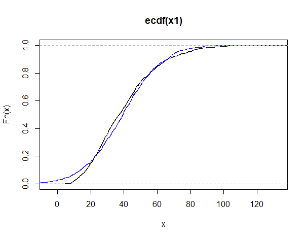
Empirical CDF (ECDF) plots look somewhat similar, but do show that the normal sample (blue) takes negative values. The K-S statistic $D$
is the maximum vertical distance between the two plots.
plot(ecdf(x1))
lines(ecdf(x2), col="blue")

It is not surprising that a Welch 2-sample t test fails to find
a difference between means and that a 2-sample F test fails to find a difference between variances. (There are no differences to be found in either test, and both tests assume both samples are normal.)
t.test(x1, x2)$p.val
[1] 0.5248905
var.test(x1, x2)$p.val
[1] 0.7486433
Moreover, smaller samples from the same two distributions are
not detected as different by the K-S test, while boxplots
hint that the distributions are not the same. [The two-sample K-S test is not known for excellent power.]
set.seed(2021)
y1 = rgamma(100, 4, .1)
y2 = rnorm(100, 40, 20)
ks.test(y1,y2)$p.val
[1] 0.05410262

Also, the K-S test had trouble distinguishing between
two samples of a thousand observations from a gamma distribution
with shape parameter 6 and a normal population with matching
means and standard deviations. [Not shown.] A gamma distribution with shape parameter 6 is somewhat less skewed than one with shape parameter 4.


