Why does $\mu > 0$ (or even $\mu > \epsilon$) "seem easier” to substantiate than $\mu \neq 0$?

Question

Consider a random variable $X$ following a normal distribution $N(\mu,\sigma^2)$. Suppose that we have drawn iid samples of $X$, obtaining a data set with a sample mean $\bar{x}>0$.

We want to test whether the data supports $\mu >0$ with a significance level $\alpha \in (0,1)$. Setting \begin{equation*} H_0: \mu \le 0, \quad H_1: \mu > 0, \end{equation*} we examine the $p$-value \begin{equation*} p \;=\; \Pr(\overline{X} \;\ge\; \bar{x} \mathrel{|} H_0) \;=\; \Pr(\overline{X} \ge \bar{x}\mathrel|{\mu \le 0}) \;\le\; \Pr(\overline{X} \ge \bar{x} \mathrel{|} \mu = 0). \end{equation*}

[N.B.: As kindly pointed out by @dimitriy, in practice we often set the null hypothesis simply to $\mu=0$, for which the $p$-value would be directly the RHS of the above inequality.]

As in textbooks, the data provides a sufficient evidence to substantiate $\mu > 0$ if $p \le \alpha$.

Now, we change our mind and test whether the data supports $\mu \neq 0$, with \begin{equation*} \hat{H}_0: \mu = 0, \quad \hat{H}_1: \mu \neq 0, \end{equation*} and the $p$-value being \begin{equation*} \hat{p} \;=\; \Pr(|\overline{X}| \ge \bar{x} \mathrel{|} \hat{H}_0) \;=\; \Pr(|\overline{X}| \ge \bar{x} \mathrel|{\mu = 0}). \end{equation*}

Again, textbooks tell us that the data provides sufficient evidence to substantiate $\mu \neq 0$ if $\hat{p} \le \alpha$, with $\alpha$ being the aforementioned significance level.

Here comes the part that confuses me. Since $$\hat{p} \ge 2p,$$ it turns out "easier" to substantiate $\mu >0$ than $\mu \neq 0$, in the sense that the data may strongly support $\mu >0$, but does not constitute sufficient evidence for $\mu \neq 0$; equivalently, the data may strongly suggest rejecting $\mu \le 0$ without being able to reject $\mu = 0$. For instance, imagine that $p \le 0.6\%$, $\hat{p} = 1.2\%$, and $\alpha = 1\%$.

[Update: We can strengthen the above observation a bit: there exists an $\epsilon >0$ that it “seems easier” to substantiate $\mu > \epsilon$ than doing the same for $\mu \neq 0$.]

So what is the logic? What have I overlooked or misunderstood? I believe the calculation is trivial to everyone here, but there seems to be something to say about the interpretation. What is it?

In my textbook, hypothesis testing is compared to a court trial, with the null hypothesis being the suspect is innocent. Following this comparison, a probably quite poor metaphor for the paradox elaborated above is that we may have strong evidence to support that "A killed B by stabbing a dagger into B's chest", but not enough justification to substantiate that "A killed B". No, I must have made some silly mistake.

Thank you very much.

Background: Being not a statistician by any means, I am asked to teach a course that involves a part of statistics. The question occurs to me when I am preparing my notes.

Answer 1

There are some misconceptions in your question that I need to clear up before getting to the answer.

The null hypothesis $H_0$ in a statistical test is always the claim you want to argue against. The alternative hypothesis $H_1$ is the claim you hope to be true.

The null and the alternative need to be

1. mutually exclusive (no overlap)
2. collectively exhaustive (partition the parameter space)
3. the equality sign ($=$, $\ge$, or $\le$) almost always appears in the null.

So your first test should have $H_0: \mu \le 0$ and $H_1: \mu > 0$.

Your second test should have $H_0: \mu = 0$ and $H_1: \mu \ne 0$.

The p-value is the probability of seeing the observed mean (or something even more extreme) if the null hypothesis was true. Then we apply the rule “reject the null when the p-value is small.” The basic idea is that if seeing a big mean is unlikely if the null was true, the null is likely to be false.

There is a slight complication in the first test. The null is a composite one: it's an interval rather than a single point. So we will have to calculate the probability when $\mu=0$, then when $\mu =-1$, and also everywhere else below zero, since all those points are inside the null. But that’s an infinite number of points! What we do instead is to calculate the probability at the most extreme point of the null hypothesis, closest to alternative parameter space, which is at $\mu = 0$. This means that the p-value is exact only for $\mu=0$. If $\mu<0$, then our p-value is just a conservative bound on the type I error rate (the error being finding a negative effect when there is none). In other words, if the true effect is negative, then finding a false positive result is even less likely than 5% (or whatever value of $\alpha$ your question requires). This is also the reason why statistics packages will express the one-sided null as $\mu=0$ rather than $\mu \le 0$, which is technically correct, but confusing notation.

Now for your question. For both one-sided and two-sided tests, we calculate the p-value with $\mu=0$. Suppose you observe a mean of $u>0$. With a two-sided test, you need to calculate $\Pr(\bar X \ge u \vert \mu=0)$ and $\Pr(\bar X \le -u \vert \mu=0)$, since both kinds of extreme values constitute evidence against that null.

With a one-sided test, seeing a mean that’s less than $-k$ doesn’t count as evidence against the null, so we only calculate $\Pr(\bar X \ge u \vert \mu=0)$. This is why the p-value is larger in the two-sided case, which means it’s easier to reject in the one-sided case.

Another way to put this is that a two-sided test is just two one-sided tests cobbled together (a superiority and an inferiority one).

Answer 2

the data may strongly support $\mu > 0$, but does not constitute sufficient evidence for $\mu \neq 0$

I don't know if this reasoning helps or if it is 100% correct... You accept to be wrong $\alpha$-percent of the times in hypothetical repeats of the test; for example, you accept to be wrong 5% of the times in rejecting the null.

In a two-tailed test you spread this 5% in the left-tail and in the right-tail of the test distribution. In the one-tailed test, you still accept the be wrong with the same frequency (say, 5%) but always in the same direction so you put all the 5% in the same tail.

In fact, I wouldn't say that in the one-tailed test it is easier to reject, but rather that you need less extreme values. You need less extreme values compared to the two-tailed test in order to keep the overall error rate at the same $\alpha$ level.

Your trial metaphor is interesting but perhaps is not appropriate because A killed B is not more (or less) extreme than A killed B by stabbing.

Answer 3

Hypothesis testing: why $\mu > 0$ (or even $\mu > \epsilon$) "seems easier” to substantiate than $\mu \neq 0$?

It seems easier because the one-sided t-test and two-sided t-test have different sensitivity for different values.

• The two-sided t-test has sensitivity split for both positive and negative values.
• The one-sided t-test has sensitivity for only the positive or only the negative values, and because of that will be 'easier' in substantiating a result (but only for a single side)

Below is a graph of the sensitivity or power for the two tests as a function of the true mean of the distribution. (Power is the probability that an observation is a positive result).

You can see that the one-sided test is not everywhere 'easier' than the two-sided test. It is only 'easier' for the positive values.

---

Also note that the tests have an equal $5\%$ probability/frequency of a positive result when in reality the effect is negative (when the true mean is equal to zero). So if the true mean is equal to zero then the two hypothesis tests are equally 'easy' in making a false claim of substantiating an alternative hypothesis (like $\mu \neq 0$ or $\mu > 0$).

But they are still different. They will make these (false) claims for different observations and for a specific observation they are not equally 'easy'.

This can occur because there is no unique way to compute p-values and associated hypothesis tests. The p-values based on different methods can be different for a particular observation but on average (for all possible observations) they will be equal.

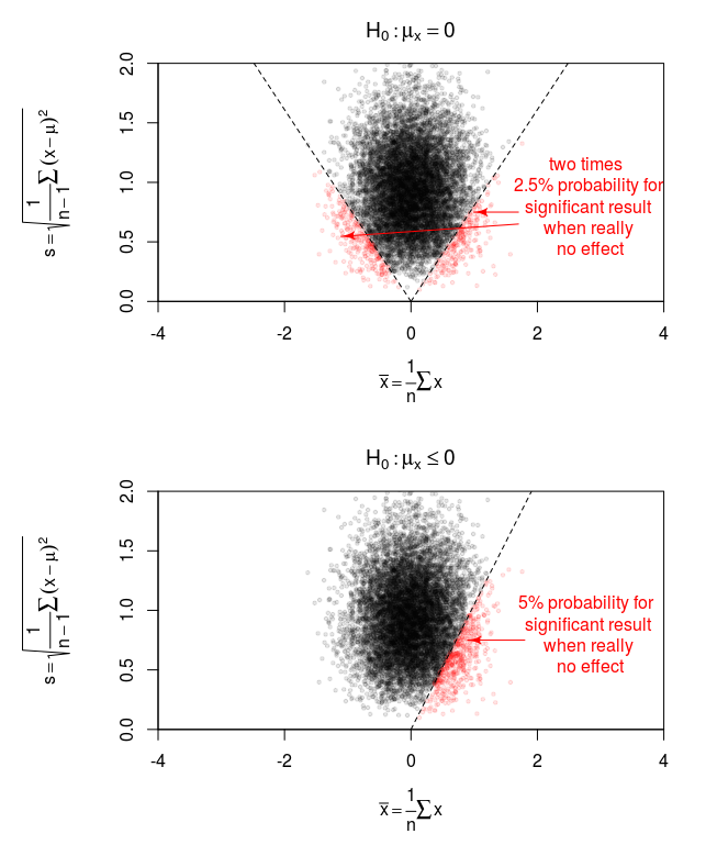
Below you see a simulation of $10 000$ samples of size $n=5$ drawn from a standard normal distribution. We plot the observed (unbiased) sample standard deviation $s$ and the observed sample mean. Along with it we plot the rejected sampled based on a two-sided t-test and a one-sided t-test.

• The amount of rejected samples is in both cases the same, namely $5\%$.
• But, the rejected samples are different for the cases. The one-sided t-test is more sensitive to values on one side. The two-sided t-test splits the sensitivity to two sides.

So again, that is why the one-sided test may seem more 'easy' but that is because of the choice to place the sensitivity in a different region. It is only 'easier' for that region.

So it may occur that you reject $H_0: \mu \leq 0$ with an alternative hypothesis $H_a: \mu > 0$, but you can't reject with the same data $H_0: \mu = 0$ with an alternative hypothesis $H_a: \neq 0$.

When such situation occurs then it is seemingly a paradox. But,

• It is not purely the data that rejected the $H_0$.
• It is also your choice and it is also the alternative hypothesis that 'helps' rejecting the null hypothesis.

The same hypothesis, with the same data, can be or not be rejected, depending on your arbitrary rejection criteria.

Other examples (from this website) were different tests reject a hypothesis for different observations are:

• ANOVA with F-test vs Tukey's range test. The ANOVA test and Tukey's procedure test the same null hypothesis 'equality of means' but have different p-values for different observations because they relate to different statistics and have sensitivity in different regions. One looks at the largest difference between samples, the other at the variance.

• Mann-Whitney U test versus t-test can be used to test equality of two means. They have different p-values because the one uses the t-statistic based on the ratio of the difference in the means and the standard deviation, the other computes a statistic based on how often a value in the one sample is larger than a sample in the other sample.

• Fisher exact test with pooled versus non-pooled data. In that question the Fisher exact test had a surprising behaviour in the power being different when the data was split into groups. But, effectively this was due to using different regions where the tests are sensitive.