What is the distribution of a random linear combination of gamma random variables?

Question

Let $U\sim \mathcal U(0, 1)$ be a random variable uniformly distributed over the interval $[0, 1]$. Let $X_1, X_2\sim \Gamma(a, b)$ be two iid random variables with a Gamma distribution. Now it is straightforward to calculate the mean and variance of the random linear combination $$Y = U\cdot X_1 + (1-U)\cdot X_2,$$ which is simply $\mathbb E(Y)=\mathbb E(X_1)$ and $var(Y)=\frac23 var(X_1)$. However, it would be very interesting for me to know the precise distribution of $Y$ but I didn't find any result for this particular problem. Does anyone know what the distribution is of $Y$?

Answer 1

A direct attack (via integration) on computing the density looks intractable.

Instead, we may more easily compute the characteristic function of $Y$ (when the scale factor $b=1,$ which we may assume without any loss of generality simply by changing the units in which we express $Y$) as

$$\begin{aligned} \phi_Y(t;a) &= E\left[e^{itY}\right] = E\left[e^{it(UX_1+(1-U)X_2)}\right] = E_U\left[E_{X_1,X_2}\left[e^{it(UX_1+(1-U)X_2)}\right]\right]\\ &= E_U\left[ E_{X_1} \left[e^{it UX_1}\right]\, E_{X_2} \left[e^{it (1-U)X_2}\right]\right]\\ &= E_U\left[(1 - i U t)^{-a}\, (1 - i(1-U)t)^{-a}\right]\\ &= \int_0^1 \left((1 - iut)(1 - i(1-u)t)\right)^{-a}\,\mathrm{d}u\\ &= \frac{_2F_1\left(1, 2-2a, 2-a; \frac{i}{2i+t}\right)\ {-}\ _2F_1\left(1, 2-2a, 2-a; \frac{i+t}{2i + t}\right)}{(a-1)t(2i + t)(1 - it)^{a-1}}. \end{aligned}$$

The hypergeo library for R will efficiently compute these hypergeometric functions, as shown in these graphs of $\phi_Y$ for a range of $a.$

The solid graph plots the real part of $\phi_Y$ and the dotted graph plots its imaginary part.

(There is a technical problem: the foregoing formula is not defined for positive integral values of $a.$ You can get close enough by computing the average of $\phi_Y(t;a\pm2\epsilon)$ when $a$ is within $\epsilon$ of an integer and $\epsilon$ is small. It doesn't have to be terribly small for this to be highly accurate; I used $\epsilon = 10^{-5}.$ Smaller values will cause too much loss of precision in double precision floating point calculations.)

That answers the question. However, often it's more useful to have a density or distribution function. Either can be obtained through a Fourier transform. The density, for instance, is

$$f_Y(y;a) = \frac{1}{2\pi}\int_{\mathbb R} e^{- i y t} \phi_Y(t;a)\,\mathrm{d}t.$$

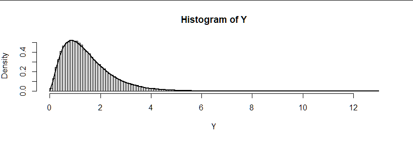
Numerical integration is possible, albeit a little slow for small values of $a.$ For $a=3/2$ it took half a minute to generate 101 points on the curve below, which matches the histogram of 100,000 values of $Y$ generated directly from its definition.

For $a=6$ the time dropped to four seconds; for $a=7.5$ to under half a second; etc. The timing is a rather irregular function of $a$ (odd multiples of $1/2$ tend to be very quick to compute) so take some care if you need many evaluations of $f_Y.$

This is the full R code.

#
# The characteristic function of Y.
#
library(hypergeo)
phi. <- function(t, a) {
  (hypergeo(1, 2 - 2*a, 2 - a, 1.i / (2.i + t)) -
     hypergeo(1, 2 - 2*a, 2 - a, (1.i + t) / (2.i + t))) /
    (t * (2.i + t) * (1 - 1.i * t)^(a-1) * (1 - a))
}
phi <- function(t, a, eps=1e-5) {
  ifelse(t == 0, 1, 
         if(isTRUE(abs(a - round(a)) > eps)) phi.(t, a) else {
           (phi.(t, a - 2*eps) + phi.(t, a + 2*eps)) / 2
         })
}
#
# Test `phi` by plotting it.
#
par(mfrow=c(1,3))
for (s in c(bquote(1/4), bquote(3/2), bquote(10))) {
  a <- eval(s)
  plot(c(-3,3), c(-1,1), type="n", 
       ylab="", yaxp=c(-1,1,2),
       xlab=expression(italic(t)), cex.lab = 1.5,
       main=bquote(italic(a)==.(s)), cex.main = 1.5)
  curve(Im(phi(x, a)), add=TRUE, lty = 3, n=201)
  curve(Re(phi(x, a)), add=TRUE, n=201)
}
par(mfrow=c(1,1))
#
# The density of Y.
#
f <- Vectorize(function(x, a, ...) {
  h <- function(t) Re(exp(-1.i * t * x) * phi(t, a)) / (2 * pi)
  integrate(h, -Inf, Inf, ...)$value
}, "x")
#
# Test with direct simulation of Y.
#
a <- 5/2 # Watch out for small or integral values -- integration can take time
b <- 1
n <- 1e5
X.1 <- rgamma(n, a, b)
X.2 <- rgamma(n, a, b)
U <- runif(n)
Y <- U * X.1 + (1 - U) * X.2

hist(Y, freq=FALSE, breaks=100)
system.time(
  # Many subdivisions are needed for small values of `a`.
  curve(f(x, a, subdivisions=5e3, rel.tol=1e-3, abs.tol=1e-4), n=101, lwd=2, add = TRUE)
)