0
$\begingroup$

I posted a question on Stack Overflow. But the question got closed as the person who closed it wrote that it should belong here in Stack Exchange. I'm not sure why but here is the link for the post. I'm aware of the residual plot shows the result of the estimate of the regression coefficient for the covariate over time. But does it make sense to convert the y-axis by exp() to get the anti-log HR? Or should I consider to plot the HR over time instead of converting the y-axis from the residual plot? But either way, I still don't know how to visualise the HR over time in R.
The problem I had when trying to exp() the y-axis is solved by the comment from Eonema. But the plot I get in R is not pretty at all.

The question from the previous post is as follows:

I have tried to visualise the proportional hazard (ph) assumption for my cox-ph model by plotting the smooth scaled schoenfeld residual plot. I'm working in R.

The residual plot is computed in R like this

test_ph <- cox.zph(my_cox_model, transform="identity")
plot(test_ph, resid=FALSE)

The output I get from the above code, is the y-axis representing the Beta(t) for the covariate over time (on the x-axis). However, I'm interested in having the y-axis showing the HR. I have tried to exp() the y values like in the following codes, and then plotting, but it did not work

hr <- exp(test_ph$y)
time <- test_ph$time #X-axis is names time in the test_ph 
plot(time, hr)

How can I convert the values on the y-axis to HR for the residual plot? Is it even possible to do that, or should I code a plot for plotting the HR over time instead converting the y-axis on the residual plot? If so, I still need help to code the latter in R as well.

Thanks in advance!

$\endgroup$
1
  • 1
    $\begingroup$ It might help if you showed a plot of the original scaled Schoenfeld residuals over time. Sometimes there are a few extreme values that can lead to even more extreme results after exponentiation. Many things in survival analysis are best evaluated on the log-hazard scale, like those residuals. In any event, I think that anyone who wants to know the HR estimates should be able to get them from the plot of the original scaled residuals. $\endgroup$
    – EdM
    Commented May 26 at 15:10

1 Answer 1

2
$\begingroup$

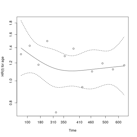
survival:::plot.cox.zph() has an argument hr which is described as follows:

if TRUE, label the y-axis using the estimated hazard ratio rather than the estimated coefficient. (The plot does not change, only the axis label.

With this example (from ?cox.zph):

library(survival)
fit <- coxph(Surv(futime, fustat) ~ age + ecog.ps, data = ovarian) 
temp <- cox.zph(fit)

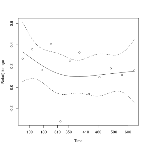
We can get the plot of $\beta(t)$ for age:

plot(temp[1])

Beta(t) for age

Or the plot of $HR(t)$ for age:

plot(temp[1], hr = TRUE)

HR(t) for age

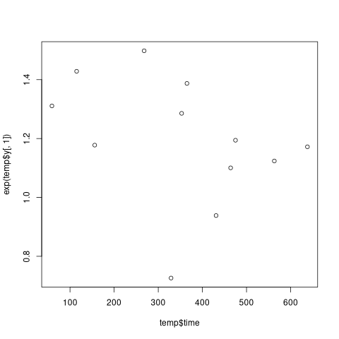
To be compared to the solution proposed on Stack Overflow:

plot(temp$time, exp(temp$y[,1]))

solution proposed on Stack Overflow

Also note this from the timedep vignette (section 4):

The cox.zph plot is excellent for diagnosis but does not, however, produce a formal fit of $\beta(t)$. What if we want to fit the model?

Two methods to fit $\beta(t)$ are then explained:

  • survsplit() for "a step function for $\beta(t)$, i.e., different coefficients over different time interval" (section 4.1);
  • the time-transform functionality of coxph (i.e. tt(...) terms in conjunction with the tt = ... argument), "If $\beta(t)$ is assumed to have a simple functional form" (section 4.2).
$\endgroup$
1
  • $\begingroup$ Please take this answer with caution! I'm very far for an expert in survival analysis and I have no formal training in statistics. I've just discovered this thanks to an answer from EdM in another question. I hope this helps! $\endgroup$
    – Thomas
    Commented Aug 11 at 14:20

Your Answer

By clicking “Post Your Answer”, you agree to our terms of service and acknowledge you have read our privacy policy.

Not the answer you're looking for? Browse other questions tagged or ask your own question.