What is the distribution of a Poisson variable, where the Poisson rate is Normal (or Binomial)?

Question

What is the distribution of $X$ if $$ X \sim \text{Poisson}(\lambda), \quad \text{where }\lambda \sim N(\mu,\sigma^2)$$

or

$$ X \sim \text{Poisson} (\lambda), \quad \text{where }\lambda \sim Bin(n,p) $$ where $n$ is very large.

Detail and motivation

In biology, next-generation sequencing is often used to quantify the level of RNA in a cell. The experiment goes like this:

Imagine that a cell (or a extract made from many cells), is a mixed bag of 200,000 RNAs molecules from 20,000 classes. We wish to estimate the proportions of the various classes.

For each replicate of an experiment we sample, with replacement, RNA "reads" from the bag.

For a class of RNA we get a count of "reads".

Each replicate of an experiment is performed with RNA from a different cell (or an extract from a different group of many cells), drawn from the same underlying population of cells.

If X is the count of "reads" from a particular replicate of the experiment, in practice we often model X as being negatively binomial as when we look at it, it looks like an overdispersed poisson.

There has been some discussion recently if their is any theoretical basis behind using the negative bionomial other than "it seems to fit". One obvious answer is that the negative binomial is the result of a poisson distribution where the poisson rate follows a gamma distribution. One interpretation is that our measurement error is poisson (counts from a sample), and the underlying variance between biological samples is gamma. But why gamma: it does not seem like an obvious answer as to the distribution to use.

A model that we are more used to might be that the amount of RNA in a sample is normally distributed (or equivalently binomially distributed with large n).

Previous attempts

I'm sure I've seen this written down somewhere before, using PGFs to figure out the result.

$$\Pi_x(s) = \sum_x{P(X=x)s^x}$$

$$P(X=x) = \int_r{P(X=x|\lambda=r)P(\lambda=r)}$$

but writing this down has only resulted in an intergral I don't know how to solve!

Answer 1

So you assume a continuous mixture of Poisson distributions, say $$ X \mid \Lambda=\lambda \sim \mathcal{Pois}(\lambda),$$ where $\Lambda$ then has some distribution on the positive line.

If we assume that $\Lambda$ has a gamma distribution, results that $X$ has a marginal negative binomial distribution. You asks what happens if $\Lambda$ has a normal distribution. That doesn't seem like a natural model since a normal distribution can take negative values, which does not make sense here. Also, the proposal of a binomial mixture distribution seems strange, since why restrict $\lambda$ to integers? Here is a review paper on continuous Poisson mixtures you could have a look at it and try some of the more prominent examples. Table 1 page 50 in the cited paper is a list of examples, many of them difficult to use due to numerical issues.

An interesting idea would be to estimate the mixing density $g$ on $(0,\infty)$ nonparametrically. There are many possible methods and many papers.

Answer 2

Normal approximation

One approach is to use a normal approximation by matching the moments.

The compound Poisson distribution is a mixture distribution of Poisson distributions with weights distributed according to a binomial distribution $w_i = P_{binom}(i\vert n,p)$

$$P(x) = \sum_{i=0}^n w_iP_{Poisson}(x\vert \lambda = i )$$

• The mean of the distribution will be equal to $$E[X] = \sum_{i=0}^n w_i E[X\vert i] = \sum w_i i = np$$ the mean of the binomial distribution.
• The variance will be $$\begin{array}{} E[(X-\mu_X)^2] &=& \sum_{i=0}^n w_i (\sigma_i^2 + \mu_i^2 - \mu^2) \\& = &\sum_{i=0}^n w_i (i + i^2 - (np)^2) \\&=& \sum_{i=0}^n w_i (i + i^2) - \sum_{i=0}^n (np)^2\\ &=& np(1-p) + (np) \end{array}$$ the variance plus the mean of the binomial distribution

Negative binomial approximation

We can do the same sort of approximation (matching the moments) with a negative binomial distribution.

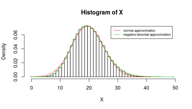
In the examples below, we have plotted this approximation as well. The curve resembles more closely the histogram than the normal approximation, but it is still not exactly the same.

Computational

The example below is computed with $n=40$ and $p=0.5$ giving $\mu_X = 20$ and $\sigma_X^2 = 30$

## parameters
set.seed(1)
ns <- 10^5
nbinom <- 40
pbinom <- 0.5

### generate sample
Y <- rbinom(ns, nbinom, pbinom)
X <- rpois(ns, Y)

### plot histogram
h <- hist(X, breaks = seq(0,max(X)+1)-0.5, freq = 0)

### add curve
xs <- seq(0,max(X)) 
#lines(xs,dpois(xs,nbinom*pbinom)*ns, col = 2)
lines(xs,dnorm(xs+0.5, mean = nbinom*pbinom, 
                     sd = sqrt(nbinom*pbinom*(2-pbinom))), col = 2)

### binomial approximation
mu = nbinom*pbinom
vr = (nbinom*pbinom*(2-pbinom))
p = 1-mu/vr
r = mu*(1-p)/p
lines(xs,dnbinom(xs, size = r, p= 1-p ), col = 3)

legend(max(X),max(h$density), c("normal approximation", "negative binomial approximation"),
       cex= 0.7, col = c(2,3),lty = 1, xjust = 1)

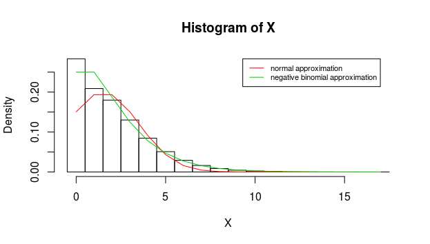
The problem with the normal approximation is that it does not work so well when $\sigma_X$ is not a lot smaller than $\mu_X$. This occurs when $\mu_X = np$ is small.

See for instance the plot below with $n=4000$ and $p=0.0005$ giving $\mu_X = 2$ and $\sigma_X^2 = 1.99975$