Is it true that the percentile bootstrap should never be used?

Question

In the MIT OpenCourseWare notes for 18.05 Introduction to Probability and Statistics, Spring 2014 (currently available here), it states:

The bootstrap percentile method is appealing due to its simplicity. However it depends on the bootstrap distribution of $\bar{x}^{*}$ based on a particular sample being a good approximation to the true distribution of $\bar{x}$. Rice says of the percentile method, "Although this direct equation of quantiles of the bootstrap sampling distribution with confidence limits may seem initially appealing, it’s rationale is somewhat obscure."[2] In short, don’t use the bootstrap percentile method. Use the empirical bootstrap instead (we have explained both in the hopes that you won’t confuse the empirical bootstrap for the percentile bootstrap).

[2] John Rice, Mathematical Statistics and Data Analysis, 2nd edition, p. 272

After a bit of searching online, this is the only quote I've found which outright states that the percentile bootstrap should not be used.

What I recall reading from the text Principles and Theory for Data Mining and Machine Learning by Clarke et al. is that the main justification for bootstrapping is the fact that $$\dfrac{1}{n}\sum_{i=1}^{n}\hat{F}_n(x) \overset{p}{\to} F(x)$$ where $\hat{F}_n$ is the empirical CDF. (I don't recall details beyond this.)

Is it true that the percentile bootstrap method should not be used? If so, what alternatives are there for when $F$ isn't necessarily known (i.e., not enough information is available to do a parametric bootstrap)?

---

Update

Because clarification has been requested, the "empirical bootstrap" from these MIT notes refers to the following procedure: they compute $\delta_1 = (\hat{\theta}^{*}-\hat{\theta})_{\alpha/2}$ and $\delta_2 = (\hat{\theta}^{*}-\hat{\theta})_{1-\alpha/2}$ with $\hat{\theta}^{*}$ the bootstrapped estimates of $\theta$ and $\hat{\theta}$ the full-sample estimate of $\theta$, and the resulting estimated confidence interval would be $[\hat{\theta}-\delta_2, \hat{\theta} - \delta_1]$.

In essence, the main idea is this: empirical bootstrapping estimates an amount proportional to the difference between the point estimate and the actual parameter, i.e., $\hat{\theta}-\theta$, and uses this difference to come up with the lower and upper CI bounds.

The "percentile bootstrap" refers to the following: use $[\hat{\theta}^*_{\alpha/2}, \hat{\theta}^*_{1-\alpha/2}]$ as the confidence interval for $\theta$. In this situation, we use bootstrapping to compute estimates of the parameter of interest and take the percentiles of these estimates for the confidence interval.

Answer 1

There are some difficulties that are common to all nonparametric bootstrapping estimates of confidence intervals (CI), some that are more of an issue with both the "empirical" (called "basic" in the boot.ci() function of the R boot package and in Ref. 1) and the "percentile" CI estimates (as described in Ref. 2), and some that can be exacerbated with percentile CIs.

TL;DR: In some cases percentile bootstrap CI estimates might work adequately, but if certain assumptions don't hold then the percentile CI might be the worst choice, with the empirical/basic bootstrap the next worst. Other bootstrap CI estimates can be more reliable, with better coverage. All can be problematic. Looking at diagnostic plots, as always, helps avoid potential errors incurred by just accepting the output of a software routine.

Bootstrap setup

Generally following the terminology and arguments of Ref. 1, we have a sample of data $y_1, ..., y_n$ drawn from independent and identically distributed random variables $Y_i$ sharing a cumulative distribution function $F$. The empirical distribution function (EDF) constructed from the data sample is $\hat F$. We are interested in a characteristic $\theta$ of the population, estimated by a statistic $T$ whose value in the sample is $t$. We would like to know how well $T$ estimates $\theta$, for example, the distribution of $(T - \theta)$.

Nonparametric bootstrap uses sampling from the EDF $\hat F$ to mimic sampling from $F$, taking $R$ samples each of size $n$ with replacement from the $y_i$. Values calculated from the bootstrap samples are denoted with "*". For example, the statistic $T$ calculated on bootstrap sample j provides a value $T_j^*$.

Empirical/basic versus percentile bootstrap CIs

The empirical/basic bootstrap uses the distribution of $(T^*-t)$ among the $R$ bootstrap samples from $\hat F$ to estimate the distribution of $(T-\theta)$ within the population described by $F$ itself. Its CI estimates are thus based on the distribution of $(T^*-t)$, where $t$ is the value of the statistic in the original sample.

This approach is based on the fundamental principle of bootstrapping (Ref. 3):

The population is to the sample as the sample is to the bootstrap samples.

The percentile bootstrap instead uses quantiles of the $T_j^*$ values themselves to determine the CI. These estimates can be quite different if there is skew or bias in the distribution of $(T-\theta)$.

Say that there is an observed bias $B$ such that: $$\bar T^*=t+B,$$

where $\bar T^*$ is the mean of the $T_j^*$. For concreteness, say that the 5th and 95th percentiles of the $T_j^*$ are expressed as $\bar T^*-\delta_1$ and $\bar T^*+\delta_2$, where $\bar T^*$ is the mean over the bootstrap samples and $\delta_1,\delta_2$ are each positive and potentially different to allow for skew. The 5th and 95th CI percentile-based estimates would directly be given respectively by:

$$\bar T^*-\delta_1=t+B-\delta_1; \bar T^*+\delta_2=t+B+\delta_2.$$

The 5th and 95th percentile CI estimates by the empirical/basic bootstrap method would be respectively (Ref. 1, eq. 5.6, page 194):

$$2t-(\bar T^*+\delta_2) = t-B-\delta_2; 2t-(\bar T^*-\delta_1) = t-B+\delta_1.$$

So percentile-based CIs both get the bias wrong and flip the directions of the potentially asymmetric positions of the confidence limits around a doubly-biased center. The percentile CIs from bootstrapping in such a case do not represent the distribution of $(T-\theta)$.

This behavior is nicely illustrated on this page, for bootstrapping a statistic so negatively biased that the original sample estimate is below the 95% CIs based on the empirical/basic method (which directly includes appropriate bias correction). The 95% CIs based on the percentile method, arranged around a doubly-negatively biased center, are actually both below even the negatively biased point estimate from the original sample!

Should the percentile bootstrap never be used?

That might be an overstatement or an understatement, depending on your perspective. If you can document minimal bias and skew, for example by visualizing the distribution of $(T^*-t)$ with histograms or density plots, the percentile bootstrap should provide essentially the same CI as the empirical/basic CI. These are probably both better than the simple normal approximation to the CI.

Neither approach, however, provides the accuracy in coverage that can be provided by other bootstrap approaches. Efron from the beginning recognized potential limitations of percentile CIs but said: "Mostly we will be content to let the varying degrees of success of the examples speak for themselves." (Ref. 2, page 3)

Subsequent work, summarized for example by DiCiccio and Efron (Ref. 4), developed methods that "improve by an order of magnitude upon the accuracy of the standard intervals" provided by the empirical/basic or percentile methods. Thus one might argue that neither the empirical/basic nor the percentile methods should be used, if you care about accuracy of the intervals.

In extreme cases, for example sampling directly from a lognormal distribution without transformation, no bootstrapped CI estimates might be reliable, as Frank Harrell has noted.

What limits the reliability of these and other bootstrapped CIs?

Several issues can tend to make bootstrapped CIs unreliable. Some apply to all approaches, others can be alleviated by approaches other than the empirical/basic or percentile methods.

The first, general, issue is how well the empirical distribution $\hat F$ represents the population distribution $F$. If it doesn't, then no bootstrapping method will be reliable. In particular, bootstrapping to determine anything close to extreme values of a distribution can be unreliable. This issue is discussed elsewhere on this site, for example here and here. The few, discrete, values available in the tails of $\hat F$ for any particular sample might not represent the tails of a continuous $F$ very well. An extreme but illustrative case is trying to use bootstrapping to estimate the maximum order statistic of a random sample from a uniform $\;\mathcal{U}[0,\theta]$ distribution, as explained nicely here. Note that bootstrapped 95% or 99% CI are themselves at tails of a distribution and thus could suffer from such a problem, particularly with small sample sizes.

Second, there is no assurance that sampling of any quantity from $\hat F$ will have the same distribution as sampling it from $F$. Yet that assumption underlies the fundamental principle of bootstrapping. Quantities with that desirable property are called pivotal. As AdamO explains:

This means that if the underlying parameter changes, the shape of the distribution is only shifted by a constant, and the scale does not necessarily change. This is a strong assumption!

For example, if there is bias it's important to know that sampling from $F$ around $\theta$ is the same as sampling from $\hat F$ around $t$. And this is a particular problem in nonparametric sampling; as Ref. 1 puts it on page 33:

In nonparametric problems the situation is more complicated. It is now unlikely (but not strictly impossible) that any quantity can be exactly pivotal.

So the best that's typically possible is an approximation. This problem, however, can often be addressed adequately. It's possible to estimate how closely a sampled quantity is to pivotal, for example with pivot plots as recommended by Canty et al. These can display how distributions of bootstrapped estimates $(T^*-t)$ vary with $t$, or how well a transformation $h$ provides a quantity $(h(T^*)-h(t))$ that is pivotal. Methods for improved bootstrapped CIs can try to find a transformation $h$ such that $(h(T^*)-h(t))$ is closer to pivotal for estimating CIs in the transformed scale, then transform back to the original scale.

The boot.ci() function provides studentized bootstrap CIs (called "bootstrap-t" by DiCiccio and Efron) and $BC_a$ CIs (bias corrected and accelerated, where the "acceleration" deals with skew) that are "second-order accurate" in that the difference between the desired and achieved coverage $\alpha$ (e.g., 95% CI) is on the order of $n^{-1}$, versus only first-order accurate (order of $n^{-0.5}$) for the empirical/basic and percentile methods (Ref 1, pp. 212-3; Ref. 4). These methods, however, require keeping track of the variances within each of the bootstrapped samples, not just the individual values of the $T_j^*$ used by those simpler methods.

In extreme cases, one might need to resort to bootstrapping within the bootstrapped samples themselves to provide adequate adjustment of confidence intervals. This "Double Bootstrap" is described in Section 5.6 of Ref. 1, with other chapters in that book suggesting ways to minimize its extreme computational demands.

---

1. Davison, A. C. and Hinkley, D. V. Bootstrap Methods and their Application, Cambridge University Press, 1997.

2. Efron, B. Bootstrap Methods: Another look at the jacknife, Ann. Statist. 7: 1-26, 1979.

3. Fox, J. and Weisberg, S. Bootstrapping regression models in R. An Appendix to An R Companion to Applied Regression, Third Edition (Sage, 2019). Revision as of 21 September 2018.

4. DiCiccio, T. J. and Efron, B. Bootstrap confidence intervals. Stat. Sci. 11: 189-228, 1996.

5. Canty, A. J., Davison, A. C., Hinkley, D. V., and Ventura, V. Bootstrap diagnostics and remedies. Can. J. Stat. 34: 5-27, 2006.

Answer 2

Some comments on different terminology between MIT / Rice and Efron's book

I think that EdM's answer does a fantastic job in answering the OPs original question, in relation to the MIT lecture notes. However, the OP also quotes the book from Efrom (2016) Computer Age Statistical Inference which uses slightly different definitions which may lead to confusion.

---

Chapter 11 - Student score sample correlation example

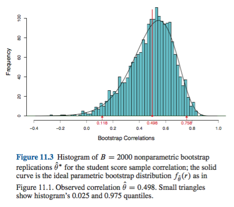
This example uses a sample for which the parameter of interest is the correlation. In the sample it is observed as $\hat \theta = 0.498$. Efron then performs $B = 2000$ non parametric bootstrap replications $\hat \theta^*$ for the student score sample correlation and plots the histogram of the results (page 186)

Standard interval bootstrap

He then defines the following Standard interval bootstrap :

$$ \hat \theta \pm 1.96 \hat{se}$$

For 95% coverage where $\hat{se}$ is taken to be the bootstrap standard error: $se_{boot}$, also called the empirical standard deviation of the bootstrap values.

Empirical standard deviation of the bootstrap values:

Let the original sample be $\mathbf{x} = (x_1,x_2,...,x_n)$ and the bootstrap sample be $\mathbf{x^*} = (x_1^*,x_2^*,...,x_n^*)$. Each bootstrap sample $b$ provides a bootstrap replication of the statistic of interest: $$ \hat \theta^{*b} = s(\mathbf{x}^{*b}) \ \text{ for } b = 1,2,...,B $$

The resulting bootstrap estimate of standard error for $\hat \theta$ is

$$\hat{se}_{boot} = \left[ \sum_{b=1}^B (\hat \theta^{*b} - \hat \theta^{*})^2 / (B-1)\right]^{1/2} $$ $$ \hat \theta^{*} = \frac{\sum_{b=1}^B \hat \theta^{*b}}{B}$$

---

This definition seems different to the one used in EdM' answer:

The empirical/basic bootstrap uses the distribution of $(T^∗−t)$ among the $R$ bootstrap samples from $\hat F$ to estimate the distribution of $(T−\theta)$ within the population described by $F$ itself.

---

Percentile bootstrap

Here, both definitions seem aligned. From Efron page 186:

The percentile method uses the shape of the bootstrap distribution to improve upon the standard intervals. Having generated $B$ replications $\hat \theta^{*1}, \hat \theta^{*2},...,\hat \theta^{*B}$ we then use the percentiles of their distribution to define percentile confidence limits.

In this example, these are 0.118 and 0.758 respectively.

Quoting EdM:

The percentile bootstrap instead uses quantiles of the $T^∗_j$ values themselves to determine the CI.

---

Comparing the standard and percentile method as defined by Efron

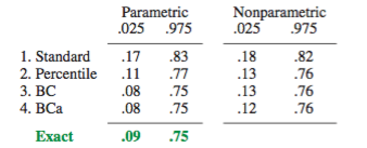
Based on his own definitions, Efron goes to considerable length to argue that the percentile method is an improvement. For this example the resulting CI are:

---

Conclusion

I would argue that the OP's original question is aligned to the definitions provided by EdM. The edits made by the OP to clarify the definitions are aligned to Efron's book and are not exactly the same for Empirical vs Standard bootstrap CI.

Comments are welcome

Answer 3

As already noted in earlier replies, the "empirical bootstrap" is called "basic bootstrap" in other sources (including the R function boot.ci), which is identical to the "percentile bootstrap" flipped at the point estimate. Venables and Ripley write ("Modern Applied Statstics with S", 4th ed., Springer, 2002, p. 136):

In asymmetric problems the basic and percentile intervals will differ considerably, and the basic intervals seem more rational.

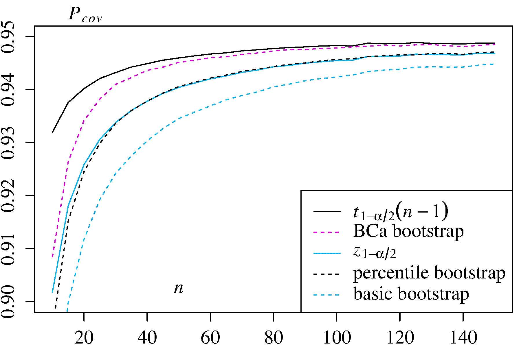
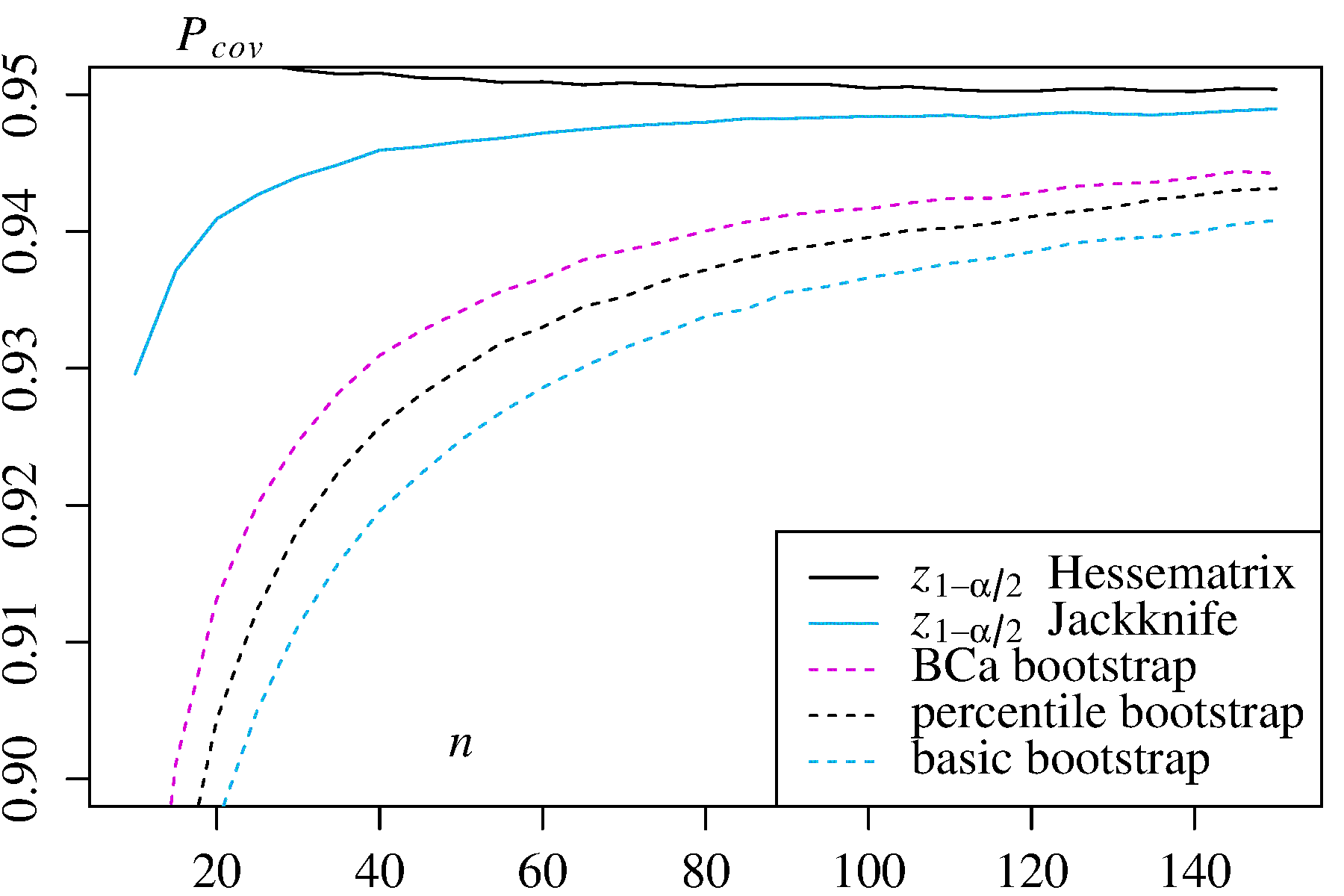
Out of curiosity, I have done extensive MonteCarlo simulations with two asymetrically distributed estimators, and found -to my own surprise- exactly the opposite, i.e. that the percentile interval outperformed the basic interval in terms of coverage probability. Here are my results with the coverage probability for each sample size $n$ estimated with one million different samples (taken from this Technical Report, p. 26f):

1. Mean of an asymmetric distribution with density $f(x)=3x^2$ In this case the classic confidence intervals $\pm t_{1-\alpha/2}\sqrt{s^2/n}$ and $\pm z_{1-\alpha/2}\sqrt{s^2/n}$ are given for comparison.

2. Maximum Likelihood Estimator for $\lambda$ in the exponential distribution In this case, two alternative confidence intervals are given for comparison: $\pm z_{1-\alpha/2}$ times the log-likelihood Hessian inverse, and $\pm z_{1-\alpha/2}$ times the Jackknife variance estimator.

In both use cases, the BCa bootstrap has the highest coverage probablity among the bootstrap methods, and the percentile bootstrap has higher coverage probability than the basic/empirical bootstrap.

Answer 4

I'm following your guideline: "Looking for an answer drawing from credible and/or official sources."

The bootstrap was invented by Brad Efron. I think it's fair to say that he's a distinguished statistician. It is a fact that he is a professor at Stanford. I think that makes his opinions credible and official.

I believe that Computer Age Statistical Inference by Efron and Hastie is his latest book and so should reflect his current views. From p. 204 (11.7, notes and details),

Bootstrap confidence intervals are neither exact nor optimal , but aim instead for a wide applicability combined with near-exact accuracy.

If you read Chapter 11, "Bootstrap Confidence Intervals", he gives 4 methods of creating bootstrap confidence intervals. The second of these methods is (11.2) The Percentile Method. The third and the fourth methods are variants on the percentile method that attempt to correct for what Efron and Hastie describe as a bias in the confidence interval and for which they give a theoretical explanation.

As an aside, I can't decide if there is any difference between what the MIT people call empirical bootstrap CI and percentile CI. I may be having a brain fart, but I see the empirical method as the percentile method after subtracting off a fixed quantity. That should change nothing. I'm probably mis-reading, but I'd be truly grateful if someone can explain how I am mis-understanding their text.

Regardless, the leading authority doesn't seem to have an issue with percentile CI's. I also think his comment answers criticisms of bootstrap CI that are mentioned by some people.

MAJOR ADD ON

Firstly, after taking the time to digest the MIT chapter and the comments, the most important thing to note is that what MIT calls empirical bootstrap and percentile bootstrap differ - The empirical bootstrap and the percentile bootstrap will be different in that what they call the empirical bootstrap will be the interval $$[\bar{x*}-\delta_{.1}, \bar{x*}-\delta_{.9}]$$ whereas the percentile bootstrap will have the confidence interval $$[\bar{x*}-\delta_{.9},\bar{x*}-\delta_{.1}].$$
I would further argue that as per Efron-Hastie the percentile bootstrap is more canonical. The key to what MIT calls the empirical bootstrap is to look at the distribution of $\delta = \bar{x} - \mu$ . But why $\bar{x} - \mu$, why not $\mu-\bar{x}$. Just as reasonable. Further, the delta's for the second set is the defiled percentile bootstrap !. Efron uses the percentile and I think that the distribution of the actual means should be most fundamental. I would add that in addition to the Efron and Hastie and the 1979 paper of Efron mentioned in another answer, Efron wrote a book on the bootstrap in 1982. In all 3 sources there are mentions of percentile bootstrap, but I find no mention of what the MIT people call the empirical bootstrap. In addition, I'm pretty sure that they calculate the percentile bootstrap incorrectly. Below is an R notebook I wrote.

Commments on the MIT reference First let’s get the MIT data into R. I did a simple cut and paste job of their bootstrap samples and saved it to boot.txt.

Hide

orig.boot = c(30, 37, 36, 43, 42, 43, 43, 46, 41, 42)
boot = read.table(file = "boot.txt")
means = as.numeric(lapply(boot,mean)) 
# lapply creates lists, not vectors.  I use it ALWAYS for data frames.
mu = mean(orig.boot)
del = sort(means - mu) # the differences
mu
means
del

And further

Hide

mu - sort(del)[3]
mu - sort(del)[18]

So we get the same answer they do. In particular I have the same 10th and 90th percentile. I want to point out that the range from the 10th to the 90th percentile is 3. This is the same as MIT has.

What are my means?

Hide
means
sort(means)

I’m getting different means. Important point- my 10th and 90th mean 38.9 and 41.9 . This is what I would expect. They are different because I am considering distances from 40.3, so I am reversing the subtraction order. Note that 40.3-38.9 = 1.4 (and 40.3 - 1.6 = 38.7). So what they call the percentile bootstrap gives a distribution that depends on the actual means we get and not the differences.

Key Point
The empirical bootstrap and the percentile bootstrap will be different in that what they call the empirical bootstrap will be the interval [x∗¯−δ.1, x∗¯−δ.9][x∗¯−δ.1, x∗¯−δ.9] whereas the percentile bootstrap will have the confidence interval [x∗¯−δ.9, x∗¯−δ.1][x∗¯−δ.9, x∗¯−δ.1]. Typically they shouldn’t be that different. I have my thoughts as to which I would prefer, but I am not the definitive source that OP requests. Thought experiment- should the two converge if the sample size increases. Notice that there are 210210 possible samples of size 10. Let’s not go nuts, but what about if we take 2000 samples- a size usually considered sufficient.

Hide

set.seed(1234) # reproducible
boot.2k = matrix(NA,10,2000)
for( i in c(1:2000)){
  boot.2k[,i] = sample(orig.boot,10,replace = TRUE)
}
mu2k = sort(apply(boot.2k, 2, mean))

Let’s look at mu2k

Hide
summary(mu2k)
mean(mu2k)-mu2k[200]
mean(mu2k) - mu2k[1801]

And the actual values-

Hide
mu2k[200]
mu2k[1801]

So now what MIT calls the empirical bootstrap gives an 80% confidence interval of [,40.3 -1.87, 40.3 +1.64] or [38.43, 41.94] and the their bad percentile distribution gives [38.5, 42]. This of course makes sense because the law of large numbers will say in this case that the distribution should converge to a normal distribution. Incidentally, this is discussed in Efron and Hastie. The first method they give for calculating the bootstrap interval is to use mu =/- 1.96 sd. As they point out, for large enough sample size this will work. They then give an example for which $n=2000$ is not large enough to get an approximately normal distribution of the data.

Conclusions Firstly, I want to state the principle I use to decide questions of naming. “It’s my party I can cry if I want to.” While originally enunciated by Petula Clark, I think it also applies naming structures. So with sincere deference to MIT, I think that Bradley Efron deserves to name the various bootstrapping methods as he wishes. What does he do ? I can find no mention in Efron of ‘empirical bootstrap’, just percentile. So I will humbly disagree with Rice, MIT, et al. I would also point out that by the law of large numbers, as used in the MIT lecture, empirical and percentile should converge to the same number. To my taste, percentile bootstrap is intuitive, justified, and what the inventor of bootstrap had in mind. I would add that I took the time to do this just for my own edification, not anything else. In particular, I didn’t write Efron, which probably is what OP should do. I am most willing to stand corrected.

Answer 5

As noted in cdalitz's answer, the percentile bootstrap gives better confidence intervals than the empirical/basic bootstrap quite often. I'd now like to offer a justification as to why this is the case.

I'm unaware of a frequentist justification for the percentile bootstrap. However, the percentile bootstrap (or a close cousin) can easily be derived from a Bayesian point of view. The Bayesian bootstrap assumes that:

1. Before observing any data, any possible data point is equally probable.
2. There is no "smoothing" of the data -- any new information or data that increases the probability of $x$ has no bearing on the probability that the next data point will equal $x + .0000...1$.
3. Let's say that we have a probability of $p$ assigned to the observed values, and a probability $1-p$ for the infinitely many values that were not observed. By an abuse of infinities that would make any mathematician cry, this means all the points not observed have a probability of $(1-p)/\infty$, i.e. 0. So we ignore any data points that did not show up in our data, and instead assume that the probability is spread out equally over the observed data. (This can be made sensible by talking about a limit of Dirichlet processes, which I'll avoid getting into here.)
4. The maximum entropy distribution to assign to the data is then a uniform distribution (more precisely, a Dirichlet distribution with $\alpha = 1$), so this is the most justifiable way to spread out the probability among the observations.

Having done this, we can simulate our posterior by drawing random frequencies for each observed value from this uniform distribution. One way to think about this is that the Bayesian bootstrap assumes the observed empirical distribution is equal to the actual likelihood function, and updates accordingly. This gives us a posterior that looks very similar to the frequentist percentile bootstrap. Some Bayesians have argued that Haldane's distribution is a less informative prior than the uniform distribution; if you use Haldane's distribution, you get the percentile bootstrap exactly. In practice the two will hardly differ for any reasonable sample size.

So if you'd like to interpret your bootstrap distribution as an approximate posterior, the percentile bootstrap does a better job than the basic/empirical bootstrap.