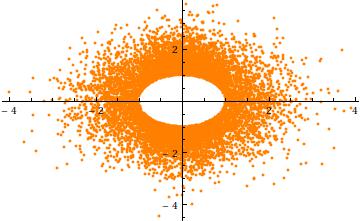
The multivariate normal distribution of $X$ is spherically symmetric. The distribution you seek truncates the radius $\rho=||X||^2$ below at $a$. Because this criterion depends only on the length of $X$, the truncated distribution remains spherically symmetric. Since $\rho$ is independent of the spherical angle $X/||X||$ and $\rho\,\sigma$ has a $\chi(n)$ distribution, you therefore can generate values from the truncated distribution in just a few simple steps:
Generate $X \sim \mathcal{N}(0,\mathbb{I}_n)$.
Generate $P$ as the square root of a $\chi^2(d)$ distribution truncated at $(a/\sigma)^2$.
Let $Y = \sigma P\, X/||X||$.
In step 1, $X$ is obtained as a sequence of $d$ independent realizations of a standard normal variable.
In step 2, $P$ is readily generated by inverting the quantile function $F^{-1}$ of a $\chi^2(d)$ distribution: generate a uniform variable $U$ supported in the range (of quantiles) between $F((a/\sigma)^2)$ and $1$ and set $P = \sqrt{F(U)}$.
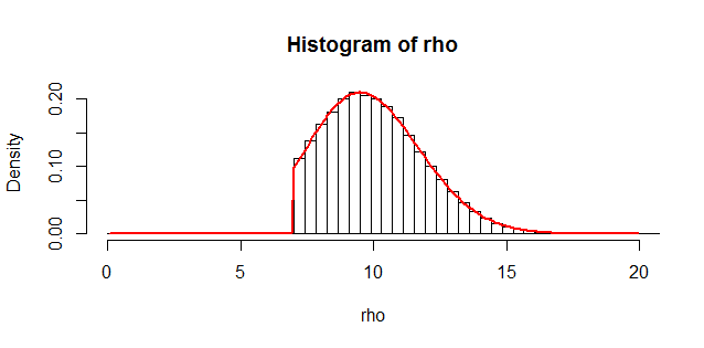
Here is a histogram of $10^5$ such independent realizations of $\sigma P$ for $\sigma=3$ in $n=11$ dimensions, truncated below at $a=7$. It took about one second to generate, attesting to the efficiency of the algorithm.

The red curve is the density of a truncated $\chi(11)$ distribution scaled by $\sigma=3$. Its close match to the histogram is evidence of the validity of this technique.
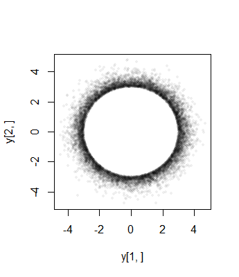
To get an intuition for the truncation, consider the case $a=3$, $\sigma=1$ in $n=2$ dimensions. Here is a scatterplot of $Y_2$ against $Y_1$ (for $10^4$ independent realizations). It clearly shows the hole at radius $a$:

Finally, note that (1) the components $X_i$ must have identical distributions (due to the spherical symmetry) and (2) except when $a=0$, that common distribution is not Normal. In fact, as $a$ grows large, the rapid decrease of the (univariate) Normal distribution causes most of the probability of the spherically truncated multivariate normal to cluster near the surface of the $n-1$-sphere (of radius $a$). The marginal distribution must therefore approximate a scaled symmetric Beta$((n-1)/2,(n-1)/2)$ distribution concentrated in the interval $(-a,a)$. This is apparent in the previous scatterplot, where $a=3\sigma$ is already large in two dimensions: the points limn a ring (a $2-1$-sphere) of radius $3\sigma$.
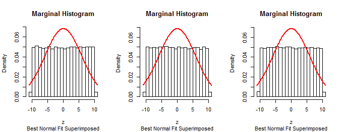
Here are histograms of the marginal distributions from a simulation of size $10^5$ in $3$ dimensions with $a=10$, $\sigma=1$ (for which the approximating Beta$(1,1)$ distribution is uniform):

Since the first $n-1$ marginals of the procedure described in the question are normal (by construction), that procedure cannot be correct.
The following R code generated the first figure. It is constructed to parallel steps 1-3 for generating $Y$. It was modified to generate the second figure by changing variables a, d, n, and sigma and then issuing the plot command plot(y[1,], y[2,], pch=16, cex=1/2, col="#00000010") after y was generated.
The generation of $U$ is modified in the code for higher numerical resolution: the code actually generates $1-U$ and uses that to compute $P$.
The same technique of simulating data according to a supposed algorithm, summarizing it with a histogram, and superimposing a histogram can be used to test the method described in the question. It will confirm that method does not work as expected.
a <- 7      # Lower threshold
d <- 11     # Dimensions
n <- 1e5    # Sample size
sigma <- 3  # Original SD
#
# The algorithm.
#
set.seed(17)
u.max <- pchisq((a/sigma)^2, d, lower.tail=FALSE)
if (u.max == 0) stop("The threshold is too large.")
u <- runif(n, 0, u.max)
rho <- sigma * sqrt(qchisq(u, d, lower.tail=FALSE))
x <- matrix(rnorm(n*d, 0, 1), ncol=d)
y <- t(x * rho / apply(x, 1, function(y) sqrt(sum(y*y))))
#
# Draw histograms of the marginal distributions.
#
h <- function(z) {
  s <- sd(z)
  hist(z, freq=FALSE, ylim=c(0, 1/sqrt(2*pi*s^2)),
       main="Marginal Histogram",
       sub="Best Normal Fit Superimposed")
  curve(dnorm(x, mean(z), s), add=TRUE, lwd=2, col="Red")
}
par(mfrow=c(1, min(d, 4)))
invisible(apply(y, 1, h))
#
# Draw a nice histogram of the distances.
#
#plot(y[1,], y[2,], pch=16, cex=1/2, col="#00000010") # For figure 2
rho.max <- min(qchisq(1 - 0.001*pchisq(a/sigma, d, lower.tail=FALSE), d)*sigma,
               max(rho), na.rm=TRUE)
k <- ceiling(rho.max/a)
hist(rho, freq=FALSE, xlim=c(0, rho.max),
     breaks=seq(0, max(rho)+a, by=a/ceiling(50/k)))
#
# Superimpose the theoretical distribution.
#
dchi <- function(x, d) {
  exp((d-1)*log(x) + (1-d/2)*log(2) - x^2/2 - lgamma(d/2))
}
curve((x >= a)*dchi(x/sigma, d) / (1-pchisq((a/sigma)^2, d))/sigma, add=TRUE,
      lwd=2, col="Red", n=257)
