29
$\begingroup$

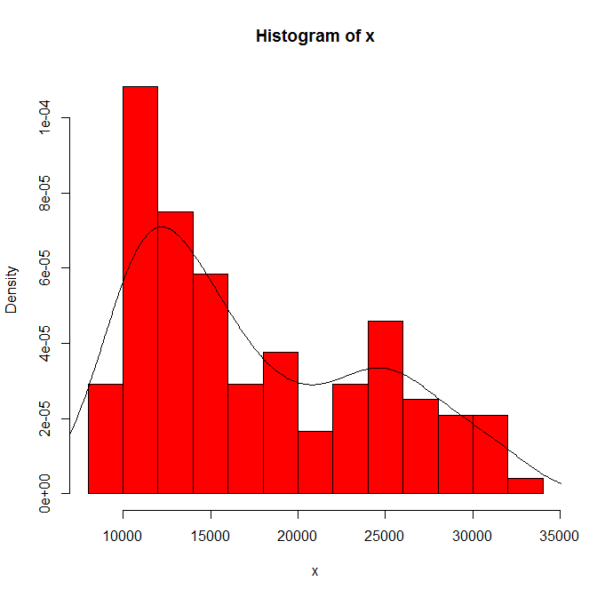
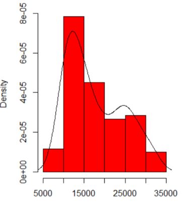
When I plot a histogram of my data, it has two peaks:

histogram

Does that mean a potential multi-modal distribution? I ran the dip.test in R (library(diptest)), and the output is:

D = 0.0275, p-value = 0.7913

I can conclude that my data have a multi-modal distribution?

DATA

10346 13698 13894 19854 28066 26620 27066 16658  9221 13578 11483 10390 11126 13487 
15851 16116 24102 30892 25081 14067 10433 15591  8639 10345 10639 15796 14507 21289 
25444 26149 23612 19671 12447 13535 10667 11255  8442 11546 15958 21058 28088 23827 
30707 19653 12791 13463 11465 12326 12277 12769 18341 19140 24590 28277 22694 15489 
11070 11002 11579  9834  9364 15128 15147 18499 25134 32116 24475 21952 10272 15404 
13079 10633 10761 13714 16073 23335 29822 26800 31489 19780 12238 15318  9646 11786 
10906 13056 17599 22524 25057 28809 27880 19912 12319 18240 11934 10290 11304 16092 
15911 24671 31081 27716 25388 22665 10603 14409 10736  9651 12533 17546 16863 23598 
25867 31774 24216 20448 12548 15129 11687 11581
$\endgroup$
3
  • 4
    $\begingroup$ Use more bins in your histogram. I suggest about twice as many $\endgroup$
    – Glen_b
    Commented Feb 19, 2015 at 5:11
  • 2
    $\begingroup$ There's mention of nine different tests in this answer, some of which may be relevant to your situation. $\endgroup$
    – Glen_b
    Commented Feb 23, 2015 at 7:15
  • 2
    $\begingroup$ This paper is likely to be useful to you, if you've not seen it already (also this follow up) $\endgroup$
    – Eoin
    Commented May 3, 2015 at 14:57

5 Answers 5

23
$\begingroup$

@NickCox has presented an interesting strategy (+1). I might consider it more exploratory in nature however, due to the concern that @whuber points out.

Let me suggest another strategy: You could fit a Gaussian finite mixture model. Note that this makes the very strong assumption that your data are drawn from one or more true normals. As both @whuber and @NickCox point out in the comments, without a substantive interpretation of these data—supported by well-established theory—to support this assumption, this strategy should be considered exploratory as well.

First, let's follow @Glen_b's suggestion and look at your data using twice as many bins:

enter image description here

We still see two modes; if anything, they come through more clearly here. (Note also that the kernel density line should be identical, but appears more spread out due to the larger number of bins.)

Now lets fit a Gaussian finite mixture model. In R, you can use the Mclust package to do this:

library(mclust)
x.gmm = Mclust(x)
summary(x.gmm)
# ----------------------------------------------------
# Gaussian finite mixture model fitted by EM algorithm 
# ----------------------------------------------------
#   
# Mclust V (univariate, unequal variance) model with 2 components:
#   
#   log.likelihood   n df       BIC       ICL
#        -1200.874 120  5 -2425.686 -2442.719
# 
# Clustering table:
#  1  2 
# 68 52 

Two normal components optimizes the BIC. For comparison, we can force a one component fit and perform a likelihood ratio test:

x.gmm.1 = Mclust(x, G=1)
logLik(x.gmm.1)
# 'log Lik.' -1226.241 (df=2)
logLik(x.gmm)-logLik(x.gmm.1)
# 'log Lik.' 25.36657 (df=5)
1-pchisq(25.36657, df=3)  # [1] 1.294187e-05

This suggests it is extremely unlikely you would find data as far from unimodal as yours if they came from a single true normal distribution.

Some people don't feel comfortable using a parametric test here (although if the assumptions hold, I don't know of any problem). One very broadly applicable technique is to use the Parametric Bootstrap Cross-fitting Method (I describe the algorithm here). We can try applying it to these data:

x.gmm$parameters
# $mean
# 12346.98 23322.06 
# $variance$sigmasq
# [1]  4514863 24582180
x.gmm.1$parameters
# $mean
# [1] 17520.91
# $variance$sigmasq
# [1] 43989870

set.seed(7809)
B = 10000;    x2.d = vector(length=B);    x1.d = vector(length=B)
for(i in 1:B){
  x2      = c(rnorm(68, mean=12346.98, sd=sqrt( 4514863)), 
              rnorm(52, mean=23322.06, sd=sqrt(24582180)) )
  x1      = rnorm( 120, mean=17520.91, sd=sqrt(43989870))
  x2.d[i] = Mclust(x2, G=2)$loglik - Mclust(x2, G=1)$loglik
  x1.d[i] = Mclust(x1, G=2)$loglik - Mclust(x1, G=1)$loglik
}
x2.d = sort(x2.d);  x1.d = sort(x1.d)
summary(x1.d)
#     Min.  1st Qu.   Median     Mean  3rd Qu.     Max. 
# -0.29070 -0.02124  0.41460  0.88760  1.36700 14.01000 
summary(x2.d)
#   Min. 1st Qu.  Median    Mean 3rd Qu.    Max. 
#  9.006  23.770  27.500  27.760  31.350  53.500 

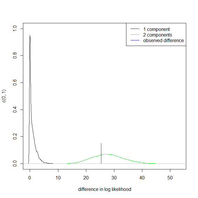
enter image description here

The summary statistics, and the kernel density plots for the sampling distributions show several interesting features. The log likelihood for the single component model is rarely greater than that of the two component fit, even when the true data generating process has only a single component, and when it is greater, the amount is trivial. The idea of comparing models that differ in their ability to fit data is one of the motivations behind the PBCM. The two sampling distributions barely overlap at all; only .35% of x2.d are less than the maximum x1.d value. If you selected a two component model if the difference in log likelihood were >9.7, you would incorrectly select the one component model .01% and the two component model .02% of the time. These are highly discriminable. If, on the other hand, you chose to use the one component model as a null hypothesis, your observed result is sufficiently small as not to show up in the empirical sampling distribution in 10,000 iterations. We can use the rule of 3 (see here) to place an upper bound on the p-value, namely, we estimate your p-value is less than .0003. That is, this is highly significant.

This raises the question of why these results diverge so much from your dip test. (To answer your explicit question, your dip test provides no evidence that there are two real modes.) I honestly don't know the dip test, so it's hard to say; it may be underpowered. However, I think the likely answer is that this approach assumes your data are generated by true normal[s]. A Shapiro-Wilk test for your data is highly significant ($p < .000001$), and it is also highly significant for the optimal Box-Cox transformation of your data (the inverse square root; $p < .001$). However, data are never really normal (cf., this famous quote), and the underlying components, should they exist, aren't guaranteed to be perfectly normal either. If you find it reasonable that your data could come from a positively skewed distribution, rather than a normal, this level of bimodality may well be within the typical range of variation, which is what I suspect the dip test is saying.

$\endgroup$
10
  • 3
    $\begingroup$ The problem with this approach is that the alternative to which you are comparing a Gaussian mixture is not very reasonable. A more reasonable one would be that the distribution is some kind of right-skewed one, such as a Gamma. It's almost a given that a mixture is going to fit almost any skewed dataset "significantly" better than a single Gaussian will fit it. $\endgroup$
    – whuber
    Commented Feb 19, 2015 at 22:27
  • $\begingroup$ You're right, @whuber. I tried to make that point explicitly. I'm not sure how to do a Gamma FMM, but that would be better. $\endgroup$ Commented Feb 19, 2015 at 22:30
  • 1
    $\begingroup$ Since this is exploratory, one thought would be to attempt to transform the original distribution to symmetry (perhaps with an offset Box-Cox transformation, robustly estimated from a few quantiles of the data) and try your approach again. Of course you wouldn't talk about "significance" per se but the analysis of the likelihood could still be revealing. $\endgroup$
    – whuber
    Commented Feb 19, 2015 at 22:34
  • $\begingroup$ @whuber, I did that, but I only mentioned it in passing. (The optimal Box-Cox transformation is the inverse square root.) You get the same result, but the p-values are (still highly, but) less significant. $\endgroup$ Commented Feb 19, 2015 at 22:40
  • 3
    $\begingroup$ I very much like the idea that you should be modelling what you think is the generating process. My problem is that even when Gaussian mixtures work well, I feel there should be a substantive interpretation. If the OP told us more even on what the data are some better guesses might be possible. $\endgroup$
    – Nick Cox
    Commented Feb 20, 2015 at 13:01
15
$\begingroup$

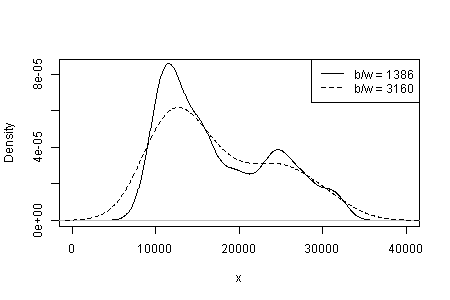
Following up on the ideas in @Nick's answer and comments, you can see how wide the bandwidth needs to be to just flatten out the secondary mode:

enter image description here

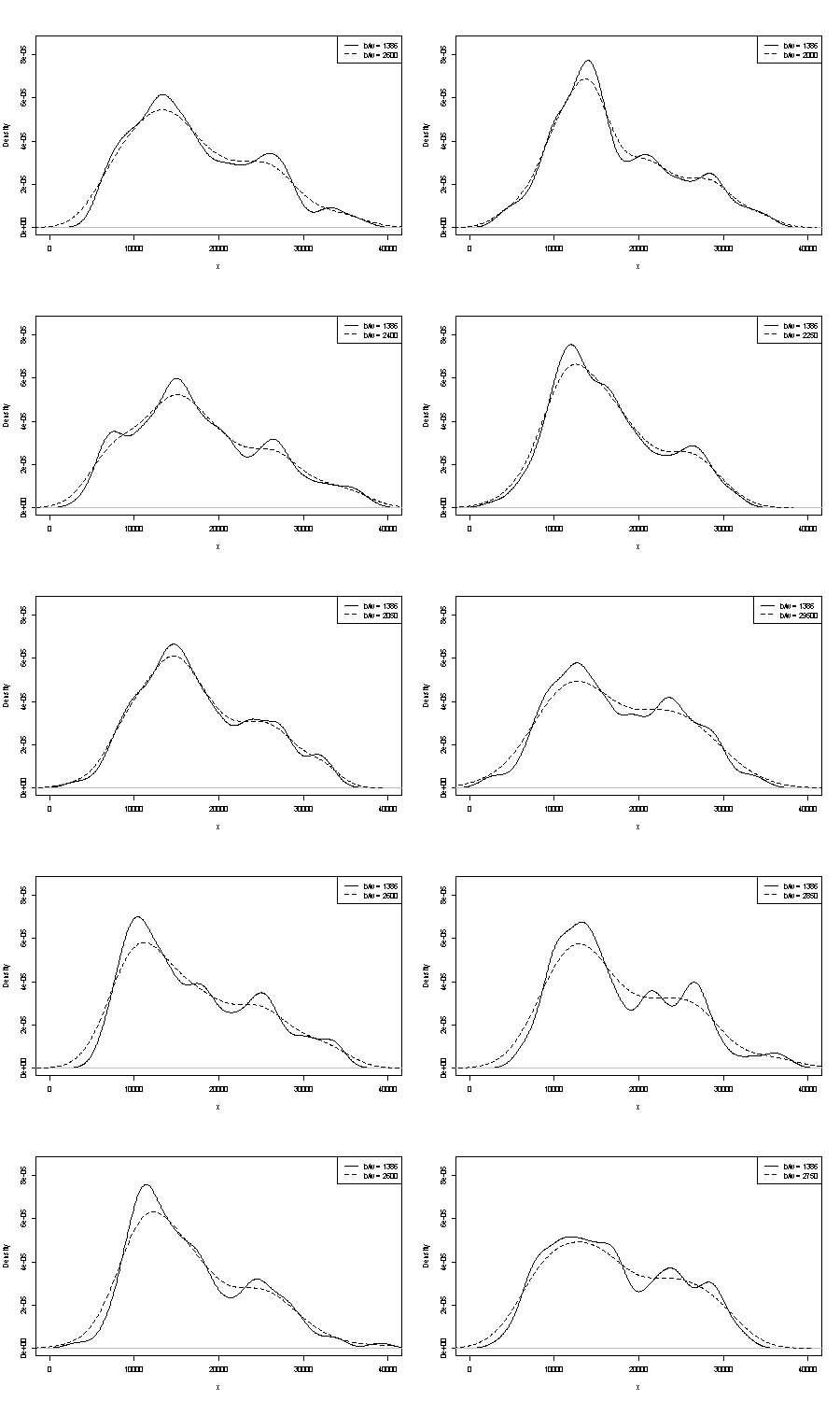
Take this kernel density estimate as the proximal null—the distribution closest to the data yet still consistent with the null hypothesis that it's a sample from a unimodal population—and simulate from it. In the simulated samples the secondary mode doesn't often look so distinct, and you needn't widen the bandwidth as much to flatten it out.

enter image description here

Formalizing this approach leads to the test given in Silverman (1981), "Using kernel density estimates to investigate modality", JRSS B, 43, 1. Schwaiger & Holzmann's silvermantest package implements this test, and also the calibration procedure described by Hall & York (2001), "On the calibration of Silverman's test for multimodality", Statistica Sinica, 11, p 515, which adjusts for asymptotic conservatism. Performing the test on your data with a null hypothesis of unimodality results in p-values of 0.08 without calibration and 0.02 with calibration. I'm not familiar enough with the dip test to guess at why it might differ.

R code:

      # kernel density estimate for x using Sheather-Jones 
          # method to estimate b/w:
    density(x, kernel="gaussian", bw="SJ") -> dens.SJ
      # tweak b/w until mode just disappears:
    density(x, kernel="gaussian", bw=3160) -> prox.null
      # fill matrix with simulated samples from the proximal 
      # null:
    x.sim <- matrix(NA, nrow=length(x), ncol=10)
    for (i in 1:10){
      x.sim[ ,i] <- rnorm(length(x), sample(x, size=length(x), 
                          replace=TRUE), prox.null$bw)
    }
      # perform Silverman test without Hall-York calibration:
    require(silvermantest)
    silverman.test(x, k=1, M=10000, adjust=F)
      # perform Silverman test with Hall-York calibration:
    silverman.test(x, k=1, M=10000, adjust=T)
$\endgroup$
5
  • 1
    $\begingroup$ +1. Interesting! What kernel is being used here? As I recall dimly, there are subtle reasons why Gaussian kernels should be used for formal variants of this approach. $\endgroup$
    – Nick Cox
    Commented Feb 20, 2015 at 13:01
  • $\begingroup$ @Nick: Gaussian kernel, but I can't remember if there's a compelling reason for that. Each simulated sample is rescaled, & there's a correction for a conservative bias the original test has - worked out by someone called Storey I think. $\endgroup$
    – Scortchi
    Commented Feb 20, 2015 at 13:23
  • $\begingroup$ @Scortchi, I tweaked your text & code slightly. I hope you don't mind. +1. Also, you use the dreaded right arrow assignment operator?! Oh the humanity... $\endgroup$ Commented Feb 20, 2015 at 14:46
  • $\begingroup$ @gung: Not at all - thank you! But is -> not best practice for some reason? $\endgroup$
    – Scortchi
    Commented Feb 20, 2015 at 15:13
  • 3
    $\begingroup$ It's no better or worse, really, but the convention in programming is to state your variables at the left & have what is assigned to them to the right. Lots of people are freaked out by ->; I'm just bemused. $\endgroup$ Commented Feb 20, 2015 at 15:20
10
$\begingroup$

The things to worry about include:

  1. The size of the dataset. It is not tiny, not large.

  2. The dependence of what you see on histogram origin and bin width. With only one choice evident, you (and we) have no idea of sensitivity.

  3. The dependence of what you see on kernel type and width and whatever other choices are made for you in density estimation. With only one choice evident, you (and we) have no idea of sensitivity.

Elsewhere I have suggested tentatively that credibility of modes is supported (but not established) by a substantive interpretation and by the ability to discern the same modality in other datasets of the same size. (Bigger is better too....)

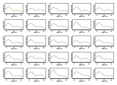
We can't comment on either of those here. One small handle on repeatability is to compare what you get with bootstrap samples of the same size. Here are the results of a token experiment using Stata, but what you see is arbitrarily limited to Stata's defaults, which themselves are documented as plucked out of the air. I got density estimates for the original data and for 24 bootstrap samples from the same.

The indication (no more, no less) is what I think experienced analysts would just guess any way from your graph. The left-hand mode is highly repeatable and the right-hand is distinctly more fragile.

Note that there is an inevitability about this: as there are fewer data nearer the right-hand mode, it won't always reappear in a bootstrap sample. But this is also the key point.
enter image description here

Note that point 3. above remains untouched. But the results are somewhere between unimodal and bimodal.

For those interested, this is the code:

clear 
set scheme s1color 
set seed 2803 

mat data = (10346, 13698, 13894, 19854, 28066, 26620, 27066, 16658, 9221, 13578, 11483, 10390, 11126, 13487, 15851, 16116, 24102, 30892, 25081, 14067, 10433, 15591, 8639, 10345, 10639, 15796, 14507, 21289, 25444, 26149, 23612, 19671, 12447, 13535, 10667, 11255, 8442, 11546, 15958, 21058, 28088, 23827, 30707, 19653, 12791, 13463, 11465, 12326, 12277, 12769, 18341, 19140, 24590, 28277, 22694, 15489, 11070, 11002, 11579, 9834, 9364, 15128, 15147, 18499, 25134, 32116, 24475, 21952, 10272, 15404, 13079, 10633, 10761, 13714, 16073, 23335, 29822, 26800, 31489, 19780, 12238, 15318, 9646, 11786, 10906, 13056, 17599, 22524, 25057, 28809, 27880, 19912, 12319, 18240, 11934, 10290, 11304, 16092, 15911, 24671, 31081, 27716, 25388, 22665, 10603, 14409, 10736, 9651, 12533, 17546, 16863, 23598, 25867, 31774, 24216, 20448, 12548, 15129, 11687, 11581)
set obs `=colsof(data)' 
gen data = data[1,_n] 

gen index = . 

quietly forval j = 1/24 { 
    replace index = ceil(120 * runiform()) 
    gen data`j' = data[index]
    kdensity data`j' , nograph at(data) gen(xx`j' d`j') 
} 

kdensity data, nograph at(data) gen(xx d) 

local xstuff xtitle(data/1000) xla(10000 "10" 20000 "20" 30000 "30") sort 
local ystuff ysc(r(0 .0001)) yla(none) `ystuff'   

local i = 1 
local colour "orange" 
foreach v of var d d? d?? { 
    line `v' data, lc(`colour') `xstuff'  `ystuff' name(g`i', replace) 
    local colour "gs8" 
    local G `G' g`i' 
    local ++i 
} 

graph combine `G' 
$\endgroup$
3
  • $\begingroup$ +1 I like your bootstrap approach: the array of plots helps everyone understand the data better. I am wondering whether those plots might be sensitive to how Stata estimates the bandwidth. I suspect that it could result in an under-powered test because its estimate probably is based on a unimodal assumption, leading to a relatively wide bandwidth. Even a slightly narrower bandwidth estimate might make the second mode more prominent in all the bootstrap samples. $\endgroup$
    – whuber
    Commented Feb 18, 2015 at 20:56
  • 2
    $\begingroup$ @whuber Thanks! As usual, you focus unerringly on the weaknesses we need to worry about, and I agree. As kernel bandwidths increase, the appearance of unimodality tends to inevitability. Conversely, small bandwidths often just indicate spurious modes that are unrepeatable and/or trivial. The trade-off truly is delicate. I think the main merit of this approach is the rhetoric of "Is that replicable if we jiggle?" I am often concerned at the willingness of software users to copy default results without reflection. $\endgroup$
    – Nick Cox
    Commented Feb 18, 2015 at 21:06
  • 2
    $\begingroup$ There are systematic approaches to this problem based on modifying bandwidth progressively and tracing the appearance and disappearance of modes as bandwidth varies. In essence, a credible mode persists and a less-than-credible mode does not. It's a cute approach, but sometimes would be firing up a tunnel constructor when a spade will do. For example, if you twiddle histogram choices and the secondary mode disappears (or moves) all too readily, don't believe it. $\endgroup$
    – Nick Cox
    Commented Feb 18, 2015 at 21:58
3
$\begingroup$

LP Nonparametric Mode Identification

LP Nonparametric Mode Identification (name of the algorithm LPMode, the ref of the paper is given below)

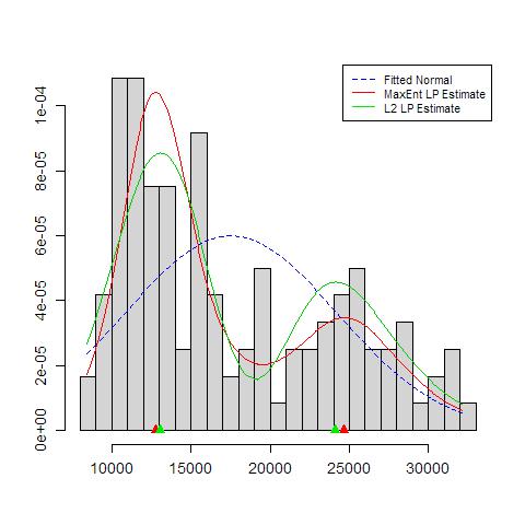
MaxEnt Modes [Red color triangles in the plot]: 12783.36 and 24654.28.

L2 Modes [Green color triangles in the plot]: 13054.70 and 24111.61.

Interesting to note the modal shapes, especially the second one which shows considerable skewness (Traditional Gaussian Mixture model likely to fail here).

Mukhopadhyay, S. (2016) Large-Scale Mode Identification and Data-Driven Sciences. https://arxiv.org/abs/1509.06428

$\endgroup$
7
  • 2
    $\begingroup$ Can you elaborate & provide some context to introduce & explain these methods? It's nice to have a link to the paper, but we prefer our answers here to be self-contained, especially if the link goes dead. $\endgroup$ Commented May 3, 2015 at 14:32
  • $\begingroup$ The context is the original question: Is there multimodality? if so positions. and relevance of a new method comes from the fact that bump hunting in a nonparametric way is hard modeling problem. $\endgroup$ Commented May 3, 2015 at 14:37
  • 2
    $\begingroup$ No, I mean what is "LP Nonparametric Mode Identification"? What is "MaxEnt"? Etc. In a couple of sentences, how does this work? Why / when might it be preferable to other methods? Etc. I am aware that you link to the paper that explains them, but it would be nice to have a couple sentences to introduce them here, especially if the link goes dead, but even if not to give future readers a sense of whether they want to pursue this method. $\endgroup$ Commented May 3, 2015 at 14:41
  • 3
    $\begingroup$ @DeepMukherjee, you certainly needn't rewrite the entire paper in your post. Just add a few sentences saying what it is & how it works. $\endgroup$ Commented May 3, 2015 at 14:42
  • 1
    $\begingroup$ @gung and Nick Cox the details of the LPMode is provided in the following arXiv paper: arxiv.org/abs/1509.06428 $\endgroup$ Commented Sep 23, 2015 at 0:20
0
$\begingroup$

I'll add that you can replace the progress bars, which don't illuminate all that much, with an iteration count instead with this:

    x2.d[i] = Mclust(x2, G=2, verbose=FALSE)$loglik - Mclust(x2, 
                     G=1, verbose=FALSE)$loglik
    x1.d[i] = Mclust(x1, G=2, verbose=FALSE)$loglik - Mclust(x1, 
                     G=1, verbose=FALSE)$loglik
    cat(sprintf("\rIteration %s of %s (%.1f%% complete)", i, B, 
              i/B*100))
$\endgroup$

Your Answer

By clicking “Post Your Answer”, you agree to our terms of service and acknowledge you have read our privacy policy.

Not the answer you're looking for? Browse other questions tagged or ask your own question.