There are already so many awesome answers here, but I'd like to share with you how I interpret the "probabilistic distribution of probabilities" as @David Robinson described in the accepted answer and add some supplementary points using some very simple illustrations and derivations.
Imagine this, we have a coin and flip it in the following three scenarios: 1) toss it five times and get TTTTT (five tails and zero head); in scenario 2) use the same coin and toss it also five times and get HTTHH (three heads and two tails); in scenario 3) get the same coin and toss it ten times and get THHTHHTHTH (six heads and four tails).
Then three issues arise a) we don't have a strategy to guess the probability in the first flipping; b) in scenario 1 the probability (we would work out) of getting head in the 6th tossing would be impossible which seems unreal(black swan event); c) in scenario 2 and 3 the (relative) probabilities of getting head next time are both $0.6$ although we know the confidence is higher in scenario 3. Therefore it is not enough to estimate the probability in tossing a coin just using a probability point and with no prior information, instead, we need a prior before we toss the coin and a probability distribution for each time step in the three cases above.
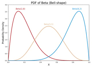
Beta distribution $\text{Beta}(\theta|\alpha_H, \alpha_T)$ can address the three problems where $\theta$ represents the density over the interval [0, 1], $\alpha_H$ the times heads occur and $\alpha_T$ the times tails occur here.
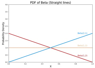
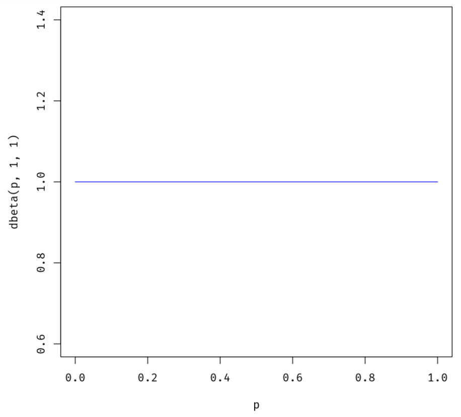
For the issue a, we can assume before flipping the coin that heads and tails are equally likely by either use a probability point and saying that the chance of occurring heads is 50%, or employing the Beta distribution and setting the prior as $\text{Beta}(\theta|1, 1)$ (equivalent to the uniform distribution) meaning two virtual tosses(we can treat the hyperparameter (1, 1) as pseudocounts) and we have observed one head event and one tail event (as depicted bellow).
p = seq(0,1, length=100)
plot(p, dbeta(p, 1, 1), ylab="dbeta(p, 1, 1)", type ="l", col="blue")
 In fact we can bridge the two methods by the following derivation:
$\begin{align*} E[\text{Beta}(\theta|\alpha_H, \alpha_T)] &= \int_0^1 \theta P(\theta|\alpha_H, \alpha_T) d\theta \hspace{2.15cm}\text{the numerator/normalization is a constant}\\
&=\dfrac{\int_0^1 \theta \{ \theta^{\alpha_H-1} (1-\theta)^{\alpha_T-1}\}\ d\theta}{B(\alpha_H,\alpha_T)}\hspace{.75cm} \text{definition of Beta; the numerator is a constant} \\
&= \dfrac{B(\alpha_H+1,\alpha_T)}{B(\alpha_H,\alpha_T)} \hspace{3cm}\text{$\theta
\theta^{\alpha_H-1}=\theta^{\alpha_H}$} \\
&= \dfrac{\Gamma(\alpha_H+1) \Gamma(\alpha_T)}{\Gamma(\alpha_H+\alpha_T+1)} \dfrac{\Gamma(\alpha_H+\alpha_T)}{\Gamma(\alpha_H)\Gamma(\alpha_T)} \\
&= \dfrac{\alpha_H}{\alpha_H+\alpha_T} \end{align*}$
We see that the expectation $\frac{1}{1+1}=50%$ is just equal to the probability point, and we can also view the probability point as one point in the Beta distribution (the Beta distribution implies that all probabilities are 100% but the probability point implies that only 50% is 100%).
For the issue b, we can calculate the posterior as follows after getting N observations(N is 5: $N_T=5$ and $N_H=0$) $\mathcal{D}$.
$\begin{align*}
\text{Beta}(\theta|\mathcal{D}, \alpha_H, \alpha_T) &\propto
P(\mathcal{D}|\theta,\alpha_H, \alpha_T)P(\theta|\alpha_H, \alpha_T) \hspace{.47cm}\text{likelihood $\times$ prior}\\
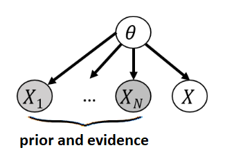
&= P(\mathcal{D}|\theta) P(\theta|\alpha_H, \alpha_T) \hspace{2cm} \text{as depicted bellow}\\
&\propto \theta^{N_H} (1-\theta)^{N_T} \cdot \theta^{\alpha_H-1} (1-\theta)^{\alpha_T-1} \\
&= \theta^{N_H+\alpha_H-1} (1-\theta)^{N_T+\alpha_T-1} \\
&= \text{Beta}(\theta|\alpha_H+N_H, \alpha_T+N_T)
\end{align*}$

$\mathcal{D}$,$\alpha_H$ and $\alpha_T$ are independent given $\theta$
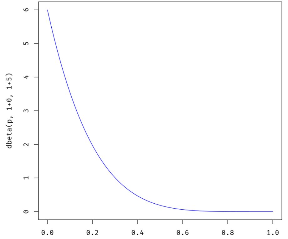
We can plug in the prior and N observations and get $\text{Beta}(\theta|1+0, 1+5)$
p = seq(0,1, length=100)
plot(p, dbeta(p, 1+0, 1+5), ylab="dbeta(p, 1+0, 1+5)", type ="l", col="blue")

We see the distribution over all probabilities of getting a head the density is high over the low probabilities but never be zero we can get otherwise, and the expectation is $E[\text{Beta}(\theta|1+0, 1+5)] = \frac{1+0}{1+0+1+5}$ (the Laplace smoothing or additive smoothing) rather than 0/impossible (in issue b).
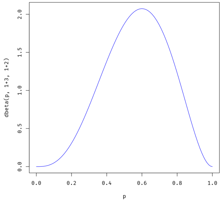
For the issue c, we can calculate the two posteriors (along the same line as the above derivation) and compare them (as with the uniform as prior). When we get three heads and two tails we get $\text{Beta}(\theta|\mathcal{D}, \alpha_H, \alpha_T)=\text{Beta}(\theta|1+3, 1+2)$
p = seq(0,1, length=100)
plot(p, dbeta(p, 1+3, 1+2), ylab="dbeta(p, 1+3, 1+2)", type ="l", col="blue")

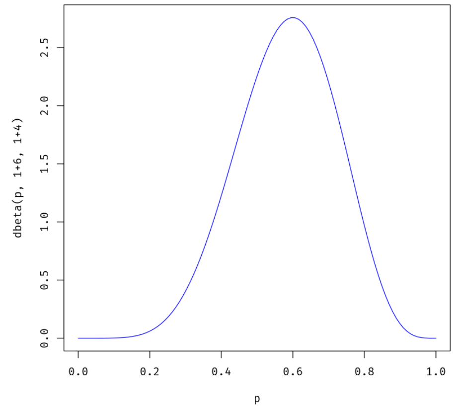
When we get six heads and four tails we get $\text{Beta}(\theta|\mathcal{D}, \alpha_H, \alpha_T)=\text{Beta}(\theta|1+6, 1+4)$
p = seq(0,1, length=100)
plot(p, dbeta(p, 1+6, 1+4), ylab="dbeta(p, 1+6, 1+4)", type ="l", col="blue")

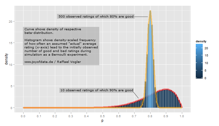
We can calculate their expectations ($\frac{1+3}{1+3+1+2} = 0.571 \approx \frac{1+6}{1+6+1+4} = 0.583$, and if we don't consider the prior $\frac{3}{3+2} = \frac{6}{6+4}$) but we can see that the second curve is more tall and narrow(more confident). The denominator of the expectation can be interpreted as a measure of confidence, the more evidence (either virtual or real) we have the more confident the posterior and the taller and narrower the curve of the Beta distribution. But if we do like that in issue c the information is just lost.
References:
- https://math.stackexchange.com/a/497599/351322
- 17.3.1.3 of Probabilistic Graphical Models Principles and Techniques
